The van der Pol problem

The van der Pol problem is a commonly used stiff test problem for ODE solvers. The stiffness is 'tunable' via modification of parameter \(\mu\) A complete reference can be found in:

    Hairer, Noersett, Wanner: Solving Ordinary Differential Equations II, p 157. Springer-Verlag 1991.

or for a practical example in Matlab, see here.

Problem Definition

The van der Pol problem can be written as a set of two first-order of non-linear ODE equations:

\begin{align} & y_1^\prime =&& y_2 \, & y_1(0) =&& y_1^\circ \nonumber \\ & y_2^\prime =&& \mu \left(1 - y_1^2\right)y_2 - y_1 \, & y_2(0) =&& y_2^\circ \nonumber \end{align}

For our purposes, we shall use:

\begin{align} y_1^\circ &= 2 \nonumber \\ y_2^\circ &= 0 \nonumber \\ \mu&= 1000 \nonumber \end{align}

for comparison purposes

A Note on Indexing

C-Indexing

The format of arrays expected by accelerInt is of note.

Note

In all cases, the C-solvers operate on local copies of the state vectors and Jacobian matrix. This means that the problem index (i.e. which IVP is being solved) does not enter into vector or matrix indexing.

The expected Jacobian ordering for the C-solvers follows pyJac v1's jacobian pattern, that is:

\begin{align} \mathcal{J}_{i, j} &= \frac{ \partial y_i^\prime } { \partial y_j } \end{align}

Pratically speaking, for the van der Pol problem, this translates to the Jacobian:

\begin{align} \mathcal{J} & = \left[ \begin{array}{cc} \frac {\partial y_1^\prime } {\partial y_1} & \frac {\partial y_1^\prime } {\partial y_2} \\ \frac {\partial y_2^\prime } {\partial y_1} & \frac {\partial y_2^\prime } {\partial y_2} \end{array} \right] \end{align}

This is then flattened in column-major (F) order, such that the flatten Jacobian array reads:

\begin{align} \vec{\mathcal{J}} & = \left\{ \frac {\partial y_1^\prime } {\partial y_1}, \frac {\partial y_2^\prime } {\partial y_1}, \frac {\partial y_1^\prime } {\partial y_2}, \frac {\partial y_2^\prime } {\partial y_2} \right\} \end{align}

This ordering can be seen in action in van_der_pol.eval_jacob()

CUDA indexing

For CUDA, the state-vector and Jacobian arrays remain in global memory by necessity due to limitations on the size of local memory per-thread. Here, the IVP index does factor into indexing concerns, and can be accessed using the built-in CUDA thread indexing parameters (e.g. threadIdx.x, etc.).

Note

Convienience macros are defined in gpu_macros.cuh to aid indexing; for an example of Jacobian layout and indexing for the CUDA-case, see jacob.cu.

Let's say we are solving \(N_{p}\) separate problems (e.g., differing initial conditions, stiffness parameter, etc.). Our Jacobian is now transformed to:

\begin{align} \mathcal{J}_{n, i, j} &= \frac{ \partial y_{n, i}^\prime } { \partial y_{n, j} } \end{align}

where \(y_{n, i}$\) is the i-th entry in the state vector of the n-th problem. Our Jacobian is again flattened in column major order, such that the flat vector is:

\begin{align} \vec{\mathcal{J}} & = \left\{ \frac {\partial y_{1, 1}^\prime } {\partial y_{1, 1}}, \frac {\partial y_{2, 1}^\prime } {\partial y_{2, 1}}, \ldots, \frac {\partial y_{N_{p}, 1}^\prime } {\partial y_{N_{p}, 1}}, \frac {\partial y_{1, 2}^\prime } {\partial y_{1, 1}}, \frac {\partial y_{2, 2}^\prime } {\partial y_{2, 1}}, \ldots \frac {\partial y_{N_{p}, 2}^\prime } {\partial y_{N_{p}, 1}}, \frac {\partial y_{1, 2}^\prime } {\partial y_{1, 1}}, \ldots \frac {\partial y_{N_{p}, 2}^\prime } {\partial y_{N_{p}, 2}} \right\} \end{align}

See also

INDEX, gpu_macros.cuh, jacob.cu

Implementation

This section details the implementation files required for the C and CUDA solvers.

RHS implementation

First, both languages need a dydt() function implementation. Both a header and implementation file are required.

• For the C-solvers, the implementation is in dydt.c and the header definition in dydt.h
• For the CUDA-sovlers, the implementation and headers are dydt.cu and dydt.cuh respectively.

Jacobian

If FINITE_DIFFERENCE is not specified in the SCons Options, an analytical Jacobian implementation must be must be specified. Both a header and implementation file are required:

• See jacob.h and jacob.c for the C-solvers
• See jacob.cuh and jacob.cu for the C-solvers

System Header

The ODE header.h file contains several important macros and definitions.

• First, the macro NSP defines the number of variables in the state vector, i.e. 2 for this problem.
• Second the macro NN should be defined to be equal to NSP. See Initial Conditions for more information.

The header.h file also contains header definitions for several functions dealing with initial conditions, set_same_initial_conditions(), apply_mask() and apply_reverse_mask().

The CUDA header.cuh file is similar to the C-version, with a few additional methods regarding GPU Memory Initialization. It contains the mechanism_memory struct, which defines memory needed for RHS and Jacobian evaluation, as well as the initialize_gpu_memory(), free_gpu_memory(), and required_mechanism_size() methods, which initialize, free and calculate the required GPU memory respectively.

GPU Memory Initialization

In order to operate the CUDA solvers, the user must implement some additional functions designed to properly initialize the required GPU memory. accelerInt pre-allocates the required memory for the solver and ODE model in the GPU's global memory to get around use of local per-thread (stack) memory allocation which becomes limiting for large ODE systems.

• required_mechanism_size() determines the amount of memory (in bytes) required per each individual CUDA thread. This is used to determine the maximum number of threads that can be launched per GPU and to split integration into batches if necessary. This is similar to the various required_solver_size() implementations for the solvers.
• initialize_gpu_memory() initializes the host and device versions of the mechanism_memory structs, similar to the various initialize_solver() implementations for the GPU solvers
• free_gpu_memory() cleans up the host and device mechanism_memory structs as with the cleanup_solver() implementation for each GPU solver.

GPU Launch Bounds

The launch_bounds.cuh file contains definitions for a few variables that control CUDA kernel launches:

• TARGET_BLOCK_SIZE defines the number of threads per CUDA block
• SHARED_SIZE defines the size of shared memory per CUDA block. This is not currently used by the solvers, but could potentially be used by a used defined RHS / Jacobian implementation.
• PREFERL1 tells CUDA to prefer a larger L1 cache over more shared memory. It is recommended to keep this on.

Initial Conditions

The initial condition reader was designed with pyJac in mind, it is currently quite cumbersome to use for other data formats.

• Although this will be upgraded in future releases, currently the NN macro should be defined to be equal to NSP.

• Additionally, the initial conditions reader expects the following data format:

  \begin{align} \nonumber \text{time}, y_1, \text{parameter}, y_2,& y_3, ... y_{NSP} \text{ (State 1)}\\ \nonumber \text{time}, y_1, \text{parameter}, y_2,& y_3, ... y_{NSP} \text{ (State 2)}\\ \nonumber \vdots& \end{align}

  An example of how to write a file in this format can be found in generate_ics.py

The set_same_initial_conditions(), defined in ics.c and ics.cu defines a simple function to set the initial conditions of the state vector if the SCons option SAME_IC is used.

• In this case, we use this method to set the initial conditions described in Problem Definition.

Additionally, ics.c / ics.cu defines the dummy methods apply_mask() and apply_reverse_mask(), which are not used for the van der Pol problem.

See also

read_initial_conditions.c, read_initial_conditions.cu

Matrix-Vector Multiplier

Finally, the sparse_multiplier.c, sparse_multiplier.cu, sparse_multiplier.h and sparse_multiplier.cuh provide headers and definitions for a "sparse" (unrolled) matrix multiplier. This is used by the exponential solvers (and may provide speedups if a sparse Jacobian is used).

Compiling the van der Pol problem.

We compile the problem with the SCons call:

    scons SAME_IC=True LOG_OUTPUT=True LOG_END_ONLY=False t_end=2000.0 t_step=1.0 mechanism_dir=examples/van_der_pol/ -j 2

This turns on the initial conditions discussed in Problem Definition.

• The j parameter allows scons to use 2 threads during compilation (vary as necessary)
• The mechanism_dir option tells scons to look in the van_der_pol example directory for Implementation implementation of the required functions described above.
• We log the output to a file (generated by default in accelerInt-root/log/solvername.bin), for plotting.
  
• The time step (t_step) is set to 1 second, while the end time (end_time) is set to 2000 seconds.
• The default error tolerances ATOL/RTOL = 10^-10 and 10^-6 respectively are used.
• Additionaly the PRINT=True option tuns on logging to the screen (if so desired)
• Alternatively, randomized initial conditions generated by generate_ics.py may be used by copying the resulting ign_data.bin file to the root accelerInt folder, and compiling without the SAME_IC option.

Running the Solvers and Plotting Results

The CPU solvers can be called using:

    ./solver_name [num_threads] [num_odes]

While the GPU solvers are called via:

    ./solver_name [num_odes]

For example, we call:

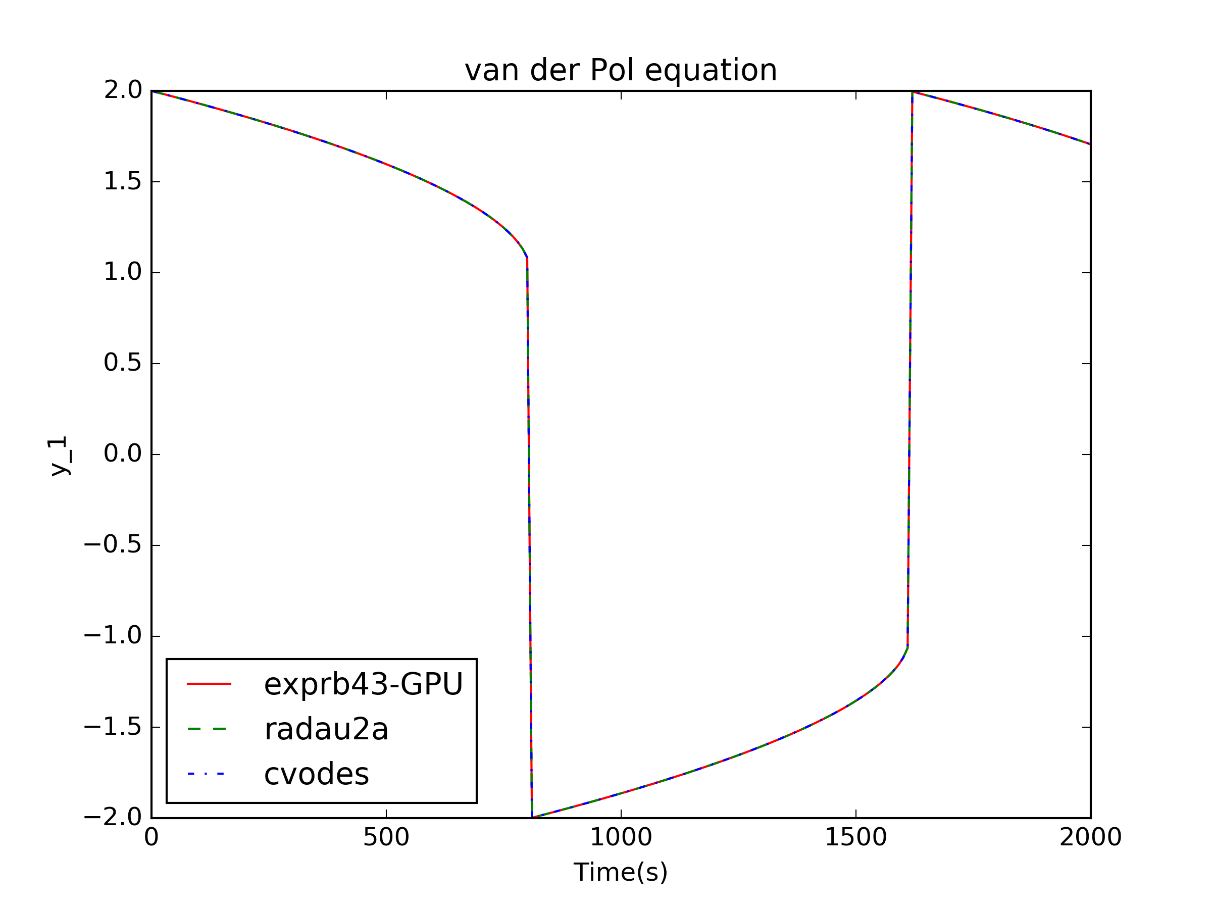
    ./exprb43-int-gpu 1
    ./cvodes-int 1 1
    ./radau2a-int 1 1

Next, we load the data and plot (plotter.py), resulting in:

Solver output for the van der Pol problem